Using multiple kernels in one Jupyter notebook

• Difficulty level: easy
• Time need to lean: 10 minutes or less
• Key points:
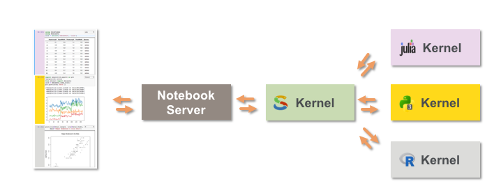
  • SoS starts and manages other jupyter kernels as subkernels
  • Each codecell belongs to either SoS or one of the subkernels
  • Subkernels can be selected from cell-level language-selection dropdown box, or SoS magics

SoS Notebook is an extension to Jupyter Notebook that allows the use of multiple kernels in one notebook. More importantly, it allows the exchange of data among subkernels so that you can, for example, preprocess data using Bash, analyze the processed data in Python, and plot the results in R. The SoS kernel is extended from the standard Python 3 kernel so you can use any Python statements in SoS. SoS Notebook is also a frontend to the SoS workflow engine but we will leave this topic to Using SoS Workflow Engine in SoS Notebook.

Installation

The SoS website has detailed instructions on how to install and run SoS Notebook in its Running SoS section.

User Interfaces

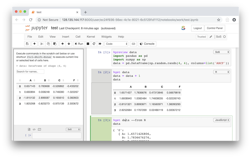
SoS Notebook is based on Jupyter and consists of the sos kernel and frontend extensions to both the classic Jupyter and Jupyter Lab. More specifically, it adds a language selection dropdown box to each code cell and a console panel to classic Jupyter. The language selection dropdown boxes are used to display and switch kernels of each code cell, and the console panel is used to execute scratch cells and display various other information generated by SoS notebook.

The following is a screenshot of a sample SoS notebook. As you can see, the three code cells are in SoS, R and JavaScript respectively,

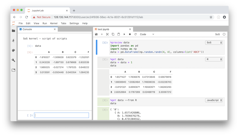
The JupyterLab interface is similar but it uses the existing console windows of JupyterLab, which does not open automatically. To get a layout similar to what is shown below, you will need to manually open a console window (right click -> Open Console for Notebook), and move it to the side if you prefer.

The SoS Notebook interface provides a number of ways to improve interactive data analysis under a Jupyter environment. For example, it allows the execution of current line (or selected text) from the current cell in the console panel so that you can step through the source code before executing the cell in its entirety. SoS also allows the displays of transient information, e.g. preview of variables in the console panel so that they do not mix with the main output. These features will be described in details in other tutorials.

Switch between kernels

The SoS kernel serves as the master kernel to other Jupyter kernels. These kernels are called subkernel and can be any Jupyter supported kernels that have been installed for Jupyter.

You can set the language of the cell to any kernel using the language drop down box to the top right corner of a code cell. For example, the following cell uses language R (kernel irkernel).

If you prefer setting the kernel explicitly in a cell, you can use magic %use. This magic starts the specified kernel and use it for the present cell.

When you create new code cell, it inherits the kernel from the code cell immediately before it. For example, the following cell uses kernel R when I insert a new code cell using the + icon on the toolbar.

To switch back to the SoS kernel, you can use the dropdown box, or magic %use SoS.

Working with subkernels

SoS can interact with any Jupyter kernel through the use of SoS kernels. Basically, SoS can

• List the kernel in the language dropdown box and use it to execute associated cells
• Use %expand magic to prepare input before sending to the kernel
• Use %capture magic to capture the output from the kernel
• Use %render magic to render output from the kernel

without knowing what the kernel does.

For example, with the variable artist defined in SoS

You can use magic %expand to create a SPARQL query with variable artist, and capture the output to another variable html_table.

Variable html_table now contains the resulting HTML table and you can parse it in Python (SoS) to extract the information.

The %render magic also captures the output from subkernels. However, instead of saving the output to a SoS variable (and process later), this magic renders the output in specified format (defult to Markdown).

For example, the usual output of the following R script would be

and you can use the %render magic to treat the text output as Markdown and be rendered in HTML

Variable exchange among subkernels

For an increasing number of kernels, SoS provides language modules to facilitate more powerful ways to work with them. The most important of which are magics to exchange variables between live kernels. Several magics can be used but the easiest and most widely used one is %get, which gets specified variables from one kernel to the present kernel.

For example, the R kernel has a mtcars dataframe and we would like to have a look at the data in Python. Then, in a SoS kernel, you can use the following magic to get the variable from R.

Note that transfer is not a correct word for what has just happened because SoS creates an independent variable with the same name, almost the same content in a similar type in the destimation kernel. What this means is that

1. The original variable is untouched.
2. A new variable in the destination kernel is created. It will have the same name as the original variable unless the original name is not allowed in the destination kernel (e.g. a R variable my.var will be transferred as my_var in Python).
3. The new variable will be in a similar type, in this case Python pandas.DataFrame for a R data.frame. This type will vary from language to language.
4. There is no gurantee of lossless data transfer because not all information could be converted between two data types in two langauges. For example, as of writing Julia's data frame type does not row label so row labels will be missing from transferred dataframes.

The %get magic uses option --from to specify the source kernel, which can be ignored if the source kernel is SoS. For example, the %get data magic executed in a R cell would get variable data from the SoS kernel.

A less popular magic is %put, which works identical to %get but goes another direction. That is to say,

Another magic that can be used to exchange variables between subkernels is %with. This magic accepts options --in (-i) and --out (-o) to pass specified input variables to the kernel, and return specified output variables from the kernel after the completion of the evaluation.

For example, if you have

you can pass the input and output variables to magic %with

and obtain the result in the SoS kernel