Examples used in Wang and Peng 2019

This vignette demonstrates how examples in the SoS workflow manuscript (Wang G. and Peng B. 2019) are reproduced.

Requirement

To run the examples, SoS workflow system have to be installed. See here for an instruction. The interactive analysis part of the RNA-seq differential expression example additionally requires one to have a Jupyter environment (Jupyter Lab or Jupyter Notebook) installed, with R kernel. Although some examples are written in *.ipynb the Jupyter format, there is no need to install notebook related software to execute those notebooks from command line (as will be shown below).

If you edit plain *.sos file with vim editor you should see customized syntax highlighting being applied to *.sos script. To use SoS Notebook as IDE to edit examples in *.ipynb format, the SoS Notebook package has to be installed. Notice that the SoS workflow system only uses SoS Notebook as the IDE and does not rely on its cross-language data communication features. So there is no need to configure SoS Notebook for different kernels if your goal is to edit and run SoS workflow system.

SoS IDE

To demonstrate SoS IDE we prepared two versions of large scale regression example:

Workflows in Jupyter format *.ipynb found on SoS live server.
- Relevant examples are under examples/WP_2019_SoS_Manuscript/WP2019_*.ipynb
Workflows in plain text *.sos found in this repository.

Jupyter-based IDE

The Jupyter version can be executed directly on our live server. Jupyter-based IDE facilicates ad hoc analysis of workflow intermediate results, inspecting the outcome and making prototype extensions of workflows.

If you want to try out the large scale regression example without installing SoS, you can run them on our live server directly. At the end of each examples/WP2019_*.ipynb file there is a cell

%sosrun

Simply execute that cell using shift-enter -- you should have activated the workflows and get results. You can use

!ls

in a new cell to list contents in the folder and examine the results.

Text-based IDE

These examples are written in plain text format SoS script. Here is a screen-shot from vim editor:

Both *.ipynb and *.sos can be executed from command line via sos run. Here we demonstrate running SoS workflow from command line with *.sos scripts.

Script specific command options

To extract narratives and possible command options from an SoS script, eg, from plain text script Process_Oriented.sos,

usage: sos run Process_Oriented.sos [workflow_name | -t targets] [options] [workflow_options]
  workflow_name:        Single or combined workflows defined in this script
  targets:              One or more targets to generate
  options:              Single-hyphen sos parameters (see "sos run -h" for details)
  workflow_options:     Double-hyphen workflow-specific parameters

Linear-model based prediction

This script fits linear models
using Lasso and Ridge regression
and summarizes their prediction performance
This script is written in process-oriented style

Workflows:
  lasso
  ridge
  default

Global Workflow Options:
  --beta 3 1.5 0 0 2 0 0 0 (as list)
                        The "true" sparse regression coefficient

Sections
  lasso_1, ridge_1:     Simulate sparse data-sets
    Workflow Options:
      --N 40 200 (as tuple)
                        training and testing samples
      --rstd 3 (as int)
      --replicate 1 2 3 4 5 (as list)
  ridge_2:              Ridge regression model implemented in R Build predictor
                        via cross-validation and make prediction
    Workflow Options:
      --nfolds 5 (as int)
  lasso_2:              LASSO model implemented in Python Build predictor via
                        cross-validation and make prediction Here I use
                        numerical indices rather than variable names for input
                        and output to demonstrate alternative syntax for
                        `_input[]` and `_output[]`
    Workflow Options:
      --nfolds 5 (as int)
  lasso_3, ridge_3:     Evaluate predictors by calculating mean squared error of
                        prediction vs truth (first line of output) and of
                        betahat vs truth (2nd line of output)
  default_1:            Run default core analysis
  default_2:            Compute and report error estimates in HTML table format

Or, for workflows in notebooks,

usage: sos run RNASeqGTEx.ipynb [workflow_name | -t targets] [options] [workflow_options]
  workflow_name:        Single or combined workflows defined in this script
  targets:              One or more targets to generate
  options:              Single-hyphen sos parameters (see "sos run -h" for details)
  workflow_options:     Double-hyphen workflow-specific parameters

Workflows:
  RNASeq_to_HDF5
  rnaseq
  peer

Sections
  RNASeq_to_HDF5:       Convert RNA-seq data to HDF5 matrices
    Workflow Options:
      --dtype 'np.uint32'
                        RNA-seq count data encoding
  rnaseq_1:             Various versions of normalization
    Workflow Options:
      --rpkm-cutoff 0.1 (as float)
                        Minimum RPKM required
      --read-cutoff 5 (as int)
                        Minimum read counts required
      --sample-cutoff 10 (as int)
                        Minimum sample counts required
  peer:                 PEER package automatic installation
  rnaseq_2:             Removing unwanted variation
    Workflow Options:
      --tissues  paths(get_output(f"h5ls {_input[2]} | awk '{{print $1}}'").strip().split('\n'))

"Process oriented" style example: feature selection in machine learning

sos run executes the SoS file *.sos. Here we demonstrate additional options to report the execution status of each step (-p) and produce the DAG to summarize execution logic (-d).

In order for these options to work, Python packages graphviz, pillow and imageio are required. They can be installed via pip install, eg, pip install graphviz pillow imageio. Additionally you need to ensure dot executable is available. Oh Debian based Linux it can be installed via

apt-get install graphviz

Of course you can choose not to bother with these dependencies by dropping the -p and -d options. They will not effect the execution of the workflow.

INFO: Running default_1: Run default core analysis
INFO: Running lasso_1: Simulate sparse data-sets
INFO: output:   data_1.train.csv data_1.test.csv... (10 items in 5 groups)
INFO: Running lasso_2: LASSO model implemented in Python Build predictor via cross-validation and make prediction Here I use numerical indices rather than variable names for input and output to demonstrate alternative syntax for `_input[]` and `_output[]`
INFO: Running ridge_1: Simulate sparse data-sets
INFO: ridge_1 (index=0) is ignored due to saved signature
INFO: ridge_1 (index=1) is ignored due to saved signature
INFO: ridge_1 (index=2) is ignored due to saved signature
INFO: ridge_1 (index=3) is ignored due to saved signature
INFO: ridge_1 (index=4) is ignored due to saved signature
INFO: output:   data_1.train.csv data_1.test.csv... (10 items in 5 groups)
INFO: Running ridge_2: Ridge regression model implemented in R Build predictor via cross-validation and make prediction
INFO: output:   data_1.lasso.predicted.csv data_1.lasso.coef.csv... (10 items in 5 groups)
INFO: Running lasso_3: Evaluate predictors by calculating mean squared error of prediction vs truth (first line of output) and of betahat vs truth (2nd line of output)
INFO: output:   data_1.lasso.mse.csv data_2.lasso.mse.csv... (5 items in 5 groups)
INFO: output:   data_1.ridge.predicted.csv data_1.ridge.coef.csv... (10 items in 5 groups)
INFO: Running ridge_3: Evaluate predictors by calculating mean squared error of prediction vs truth (first line of output) and of betahat vs truth (2nd line of output)
INFO: output:   data_1.ridge.mse.csv data_2.ridge.mse.csv... (5 items in 5 groups)
INFO: Running default_2: Compute and report error estimates in HTML table format
pandoc.css:   0%|                                      | 0/3976 [00:00<?, ?it/s]
INFO: Report saved to report.html
INFO: Workflow default (ID=2658daf4cfd433df) is executed successfully with 7 completed steps, 27 completed substeps, 1 ignored step and 5 ignored substeps.
INFO: Workflow DAG saved to Process_Oriented_011019_2251.dot
INFO: Summary of workflow saved to Process_Oriented_Report.html

Notice that each workflow step processes in parallel 5 replicates, generating 5 or 10 output files concurrently. This is what it is meant by "groups" in the output message above.

Package dependencies for this workflow

R and Python

The workflow requires R packages MASS and glmnet, and Python packages sklearn. If you do not have these packages on your system SoS will quit on error for relevant steps.

There are many ways to install these packages in R and Python. But caution that in Python to install sklearn via pip you need to type in scikit-learn instead, eg:

pip install scikit-learn==0.20.0

`pandoc` for generating reports

pandoc (version 2+) is needed to generate the HTML report.

The outcome of this workflow is a table of performance comparison, summarized in report.html. Here is the content of it:

Also available, due to -p and -d options, is a workflow status report automatically generated by the workflow. See here for the status report.

"Outcome oriented" style example: feature selection in machine learning

Here we also output status report and DAG, for comparison with the previous command.

INFO: Running simulation: Simulate sparse data-sets
INFO: Running simulation: Simulate sparse data-sets
INFO: Running simulation: Simulate sparse data-sets
INFO: Running simulation: Simulate sparse data-sets
INFO: Running simulation: Simulate sparse data-sets
INFO: output:   data_1.train.csv data_1.test.csv
INFO: output:   data_2.train.csv data_2.test.csv
INFO: output:   data_3.train.csv data_3.test.csv
INFO: output:   data_4.train.csv data_4.test.csv
INFO: Running ridge: Ridge regression model implemented in R Build predictor via cross-validation and make prediction
INFO: Running ridge: Ridge regression model implemented in R Build predictor via cross-validation and make prediction
INFO: output:   data_5.train.csv data_5.test.csv
INFO: Running lasso: LASSO model implemented in Python Build predictor via cross-validation and make prediction
INFO: Running lasso: LASSO model implemented in Python Build predictor via cross-validation and make prediction
INFO: Running ridge: Ridge regression model implemented in R Build predictor via cross-validation and make prediction
INFO: Running ridge: Ridge regression model implemented in R Build predictor via cross-validation and make prediction
INFO: Running ridge: Ridge regression model implemented in R Build predictor via cross-validation and make prediction
INFO: Running lasso: LASSO model implemented in Python Build predictor via cross-validation and make prediction
INFO: Running lasso: LASSO model implemented in Python Build predictor via cross-validation and make prediction
INFO: Running lasso: LASSO model implemented in Python Build predictor via cross-validation and make prediction
INFO: output:   data_1.lasso.predicted.csv data_1.lasso.coef.csv
INFO: Running evaluation: Evaluate predictors by calculating mean squared error of prediction vs truth (first line of output) and of betahat vs truth (2nd line of output)
INFO: output:   data_2.lasso.predicted.csv data_2.lasso.coef.csv
INFO: Running evaluation: Evaluate predictors by calculating mean squared error of prediction vs truth (first line of output) and of betahat vs truth (2nd line of output)
INFO: output:   data_1.lasso.mse.csv
INFO: output:   data_4.lasso.predicted.csv data_4.lasso.coef.csv
INFO: output:   data_3.lasso.predicted.csv data_3.lasso.coef.csv
INFO: output:   data_1.ridge.predicted.csv data_1.ridge.coef.csv
INFO: output:   data_2.lasso.mse.csv
INFO: output:   data_2.ridge.predicted.csv data_2.ridge.coef.csv
INFO: output:   data_5.lasso.predicted.csv data_5.lasso.coef.csv
INFO: Running evaluation: Evaluate predictors by calculating mean squared error of prediction vs truth (first line of output) and of betahat vs truth (2nd line of output)
INFO: Running evaluation: Evaluate predictors by calculating mean squared error of prediction vs truth (first line of output) and of betahat vs truth (2nd line of output)
INFO: Running evaluation: Evaluate predictors by calculating mean squared error of prediction vs truth (first line of output) and of betahat vs truth (2nd line of output)
INFO: Running evaluation: Evaluate predictors by calculating mean squared error of prediction vs truth (first line of output) and of betahat vs truth (2nd line of output)
INFO: Running evaluation: Evaluate predictors by calculating mean squared error of prediction vs truth (first line of output) and of betahat vs truth (2nd line of output)
INFO: output:   data_4.ridge.predicted.csv data_4.ridge.coef.csv
INFO: output:   data_3.ridge.predicted.csv data_3.ridge.coef.csv
INFO: output:   data_4.lasso.mse.csv
INFO: output:   data_1.ridge.mse.csv
INFO: output:   data_5.ridge.predicted.csv data_5.ridge.coef.csv
INFO: output:   data_2.ridge.mse.csv
INFO: output:   data_3.lasso.mse.csv
INFO: output:   data_5.lasso.mse.csv
INFO: Running evaluation: Evaluate predictors by calculating mean squared error of prediction vs truth (first line of output) and of betahat vs truth (2nd line of output)
INFO: Running evaluation: Evaluate predictors by calculating mean squared error of prediction vs truth (first line of output) and of betahat vs truth (2nd line of output)
INFO: Running evaluation: Evaluate predictors by calculating mean squared error of prediction vs truth (first line of output) and of betahat vs truth (2nd line of output)
INFO: output:   data_3.ridge.mse.csv
INFO: output:   data_5.ridge.mse.csv
INFO: output:   data_4.ridge.mse.csv
INFO: Running default: Compute and report error estimates in HTML table format
INFO: Report saved to report.html
INFO: Workflow default (ID=1dc69aff03750855) is executed successfully with 26 completed steps.
INFO: Workflow DAG saved to Outcome_Oriented_011019_2252.dot
INFO: Summary of workflow saved to Outcome_Oriented_Report.html

This workflow results in the same output as the previous one, in report.html:

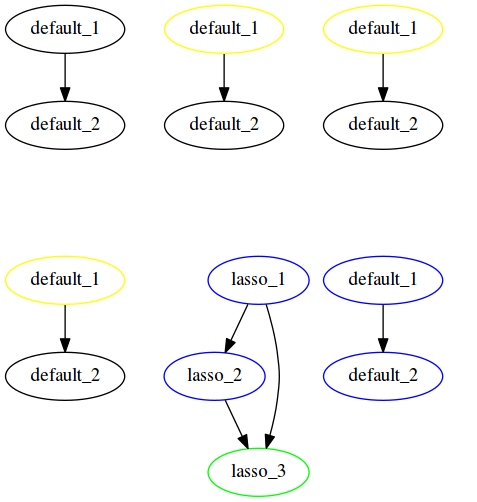
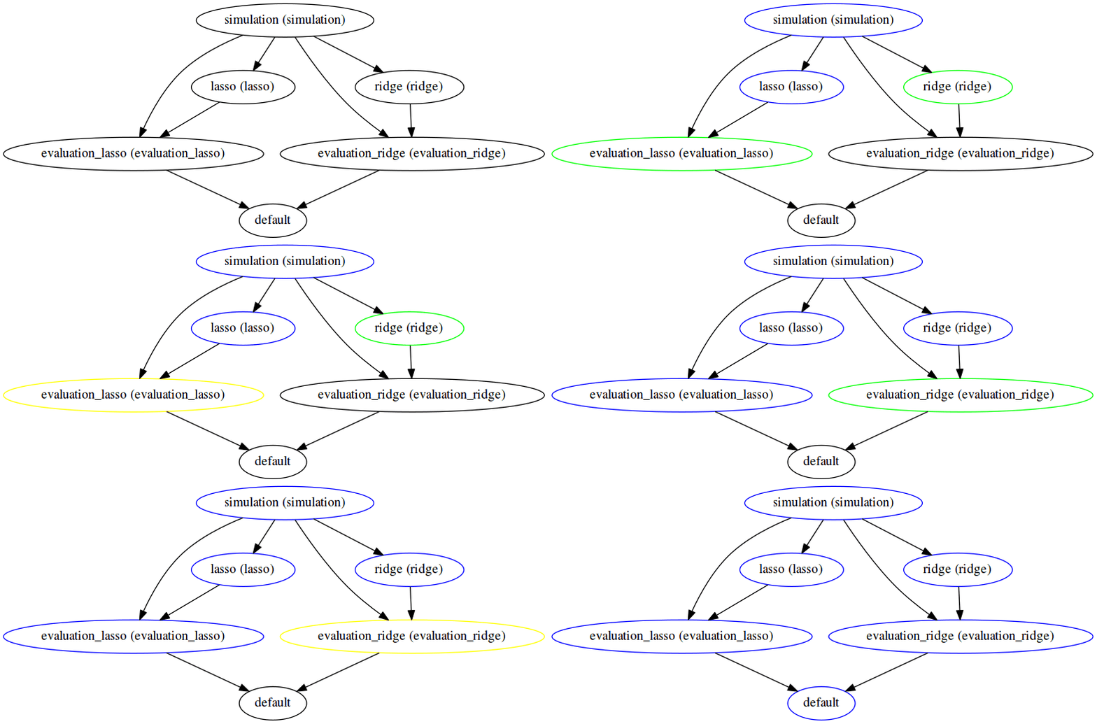
The execution graph of this style can be found in the status report generated here. Notice the difference in the DAG generated -- here all file targets are incorporated into one DAG, compared to having 2 DAGs for the previous workflow for Lasso and ridge separately.

"Mixed" style example: feature selection in machine learning

INFO: Running default: 
INFO: Running simulation: Simulate sparse data-sets
INFO: Running simulation: Simulate sparse data-sets
INFO: Running simulation: Simulate sparse data-sets
INFO: Running simulation: Simulate sparse data-sets
INFO: Running simulation: Simulate sparse data-sets
INFO: output:   data_1.train.csv data_1.test.csv
INFO: output:   data_2.train.csv data_2.test.csv
INFO: Running model fitting: LASSO model implemented in Python Build predictor via cross-validation and make prediction
INFO: Running model fitting: LASSO model implemented in Python Build predictor via cross-validation and make prediction
INFO: output:   data_3.train.csv data_3.test.csv
INFO: output:   data_4.train.csv data_4.test.csv
INFO: Running model fitting: LASSO model implemented in Python Build predictor via cross-validation and make prediction
INFO: Running model fitting: Ridge regression model implemented in R Build predictor via cross-validation and make prediction
INFO: Running model fitting: Ridge regression model implemented in R Build predictor via cross-validation and make prediction
INFO: output:   data_5.train.csv data_5.test.csv
INFO: Running model fitting: LASSO model implemented in Python Build predictor via cross-validation and make prediction
INFO: Running model fitting: LASSO model implemented in Python Build predictor via cross-validation and make prediction
INFO: Running model fitting: Ridge regression model implemented in R Build predictor via cross-validation and make prediction
INFO: Running model fitting: Ridge regression model implemented in R Build predictor via cross-validation and make prediction
INFO: output:   data_2.lasso.predicted.csv data_2.lasso.coef.csv
INFO: output:   data_1.lasso.predicted.csv data_1.lasso.coef.csv
INFO: Running model fitting: Ridge regression model implemented in R Build predictor via cross-validation and make prediction
INFO: Running evaluate: Evaluate predictors by calculating mean squared error of prediction vs truth (first line of output) and of betahat vs truth (2nd line of output)
INFO: output:   data_3.lasso.predicted.csv data_3.lasso.coef.csv
INFO: Running evaluate: Evaluate predictors by calculating mean squared error of prediction vs truth (first line of output) and of betahat vs truth (2nd line of output)
INFO: output:   data_4.lasso.predicted.csv data_4.lasso.coef.csv
INFO: Running evaluate: Evaluate predictors by calculating mean squared error of prediction vs truth (first line of output) and of betahat vs truth (2nd line of output)
INFO: Running evaluate: Evaluate predictors by calculating mean squared error of prediction vs truth (first line of output) and of betahat vs truth (2nd line of output)
INFO: output:   data_1.lasso.mse.csv
INFO: output:   data_5.lasso.predicted.csv data_5.lasso.coef.csv
INFO: output:   data_2.lasso.mse.csv
INFO: Running evaluate: Evaluate predictors by calculating mean squared error of prediction vs truth (first line of output) and of betahat vs truth (2nd line of output)
INFO: output:   data_4.lasso.mse.csv
INFO: output:   data_3.lasso.mse.csv
INFO: output:   data_5.lasso.mse.csv
INFO: output:   data_1.ridge.predicted.csv data_1.ridge.coef.csv
INFO: output:   data_2.ridge.predicted.csv data_2.ridge.coef.csv
INFO: Running ridge_2: Evaluate predictors by calculating mean squared error of prediction vs truth (first line of output) and of betahat vs truth (2nd line of output)
INFO: Running ridge_2: Evaluate predictors by calculating mean squared error of prediction vs truth (first line of output) and of betahat vs truth (2nd line of output)
INFO: output:   data_4.ridge.predicted.csv data_4.ridge.coef.csv
INFO: output:   data_3.ridge.predicted.csv data_3.ridge.coef.csv
INFO: Running ridge_2: Evaluate predictors by calculating mean squared error of prediction vs truth (first line of output) and of betahat vs truth (2nd line of output)
INFO: Running ridge_2: Evaluate predictors by calculating mean squared error of prediction vs truth (first line of output) and of betahat vs truth (2nd line of output)
INFO: output:   data_2.ridge.mse.csv
INFO: output:   data_1.ridge.mse.csv
INFO: output:   data_4.ridge.mse.csv
INFO: output:   data_5.ridge.predicted.csv data_5.ridge.coef.csv
INFO: output:   data_3.ridge.mse.csv
INFO: Running ridge_2: Evaluate predictors by calculating mean squared error of prediction vs truth (first line of output) and of betahat vs truth (2nd line of output)
INFO: output:   data_5.ridge.mse.csv
INFO: Workflow default (ID=daca32f97c9ba34c) is executed successfully with 26 completed steps and 30 completed substeps.
INFO: Workflow DAG saved to Mixed_Style_011019_2252.dot
INFO: Summary of workflow saved to Mixed_Style_Report.html

The output will be the same as previous styles, but execution graph is logically different from previous graphs, as shown in the status report here.

"Outcome oriented" style with step target dependencies

INFO: Running simulation: Simulate sparse data-sets
INFO: output:   data_1.train.csv data_1.test.csv... (10 items in 5 groups)
INFO: Running lasso: LASSO model implemented in Python Build predictor via cross-validation and make prediction
INFO: Running ridge: Ridge regression model implemented in R Build predictor via cross-validation and make prediction
INFO: output:   data_1.lasso.predicted.csv data_1.lasso.coef.csv... (10 items in 5 groups)
INFO: Running evaluation_lasso: 
INFO: Running evaluation_core: Evaluate predictors by calculating mean squared error of prediction vs truth (first line of output) and of betahat vs truth (2nd line of output)
INFO: output:   data_1.lasso.mse.csv data_2.lasso.mse.csv... (5 items in 5 groups)
INFO: output:   data_1.lasso.mse.csv data_2.lasso.mse.csv... (5 items)
INFO: output:   data_1.ridge.predicted.csv data_1.ridge.coef.csv... (10 items in 5 groups)
INFO: Running evaluation_ridge: 
INFO: Running evaluation_core: Evaluate predictors by calculating mean squared error of prediction vs truth (first line of output) and of betahat vs truth (2nd line of output)
INFO: output:   data_1.ridge.mse.csv data_2.ridge.mse.csv... (5 items in 5 groups)
INFO: output:   data_1.ridge.mse.csv data_2.ridge.mse.csv... (5 items)
INFO: Running default: 
INFO: output:   data_1.lasso.mse.csv data_2.lasso.mse.csv... (10 items)
INFO: Workflow default (ID=1764a879371ccfc7) is executed successfully with 8 completed steps and 28 completed substeps.
INFO: Workflow DAG saved to Outcome_Oriented_Step_Targets_011019_2253.dot
INFO: Summary of workflow saved to Outcome_Target_Report.html

The execution logic of outcome oriented style with step targets is the same as that of outcome oriented style with file targets. But as one can tell from the difference in DAG, the dependencies are made more explicit and the DAG representation is more abstract yet clearer.

"Mixed style" example using `named_output`

INFO: Running default: 
INFO: Running simulation: Simulate sparse data-sets
INFO: output:   data_1.train.csv data_1.test.csv... (10 items in 5 groups)
INFO: Running model fitting: LASSO model implemented in Python Build predictor via cross-validation and make prediction
INFO: Running simulation: Simulate sparse data-sets
INFO: simulation (index=1) is ignored due to saved signature
INFO: simulation (index=2) is ignored due to saved signature
INFO: simulation (index=0) is ignored due to saved signature
INFO: simulation (index=3) is ignored due to saved signature
INFO: simulation (index=4) is ignored due to saved signature
INFO: output:   data_1.train.csv data_1.test.csv... (10 items in 5 groups)
INFO: Running model fitting: Ridge regression model implemented in R Build predictor via cross-validation and make prediction
INFO: output:   data_1.lasso.predicted.csv data_1.lasso.coef.csv... (10 items in 5 groups)
INFO: Running evaluate: Evaluate predictors by calculating mean squared error of prediction vs truth (first line of output) and of betahat vs truth (2nd line of output)
INFO: output:   data_1.mse.csv data_2.mse.csv... (5 items in 5 groups)
INFO: output:   data_1.ridge.predicted.csv data_1.ridge.coef.csv... (10 items in 5 groups)
INFO: Running ridge_2: Evaluate predictors by calculating mean squared error of prediction vs truth (first line of output) and of betahat vs truth (2nd line of output)
INFO: output:   data_1.mse.csv data_2.mse.csv... (5 items in 5 groups)
INFO: Workflow default (ID=4cbde8bae0768b9a) is executed successfully with 6 completed steps, 26 completed substeps, 1 ignored step and 5 ignored substeps.
INFO: Workflow DAG saved to Mixed_Style_Data_Flow_011019_2255.dot
INFO: Summary of workflow saved to Mixed_Style_Data_Flow_Report.html

This example features the use of named_output to define dependencies for the process-oriented subworkflows. Because the dependency pattern is a lot less complicated than in Outcome Oriented style example, it can be sufficiently replaced by using a less powerful yet more intuitive implementation with named_output function.

Modular implementation of feature selection in machine learning

Examples above implemented several stand-alone *.sos scripts that contains all codes required to run the feature selection task and comparisons. Alternatively, one can created separate scripts (in R or Python in this example) to implement the core computation, and execute them in SoS. Here we give examples of such modular implementation of some pipelines above.

The module files are available under folder regression_modules. For example, the content of lasso.py is displayed below:

## python lasso.py train.txt test.txt 5 pred.txt coef.txt
import sys
import numpy as np
from sklearn.linear_model import LassoCV
train = np.genfromtxt(sys.argv[1], delimiter = ",")
test = np.genfromtxt(sys.argv[2], delimiter = ",")
model = LassoCV(cv = int(sys.argv[3]), fit_intercept = False).fit(train[:,1:], train[:,1])
Ypred = model.predict(test[:,1:])
np.savetxt(sys.argv[4], Ypred)
np.savetxt(sys.argv[5], model.coef_)

Pipelines Process_Oriented_Modular.sos and Outcome_Oriented_Modular.sos both use these modules. To run an example,

INFO: Running default_1: Run default core analysis
INFO: Running lasso_1: Simulate sparse data-sets
INFO: output:   data_1.train.csv data_1.test.csv... (10 items in 5 groups)
INFO: Running lasso_2: LASSO model implemented in Python Build predictor via cross-validation and make prediction
INFO: Running ridge_1: Simulate sparse data-sets
INFO: ridge_1 (index=0) is ignored due to saved signature
INFO: ridge_1 (index=2) is ignored due to saved signature
INFO: ridge_1 (index=1) is ignored due to saved signature
INFO: ridge_1 (index=3) is ignored due to saved signature
INFO: ridge_1 (index=4) is ignored due to saved signature
INFO: output:   data_1.train.csv data_1.test.csv... (10 items in 5 groups)
INFO: Running ridge_2: Ridge regression model implemented in R Build predictor via cross-validation and make prediction
INFO: output:   data_1.lasso.predicted.csv data_1.lasso.coef.csv... (10 items in 5 groups)
INFO: Running lasso_3: Evaluate predictors by calculating mean squared error of prediction vs truth (first line of output) and of betahat vs truth (2nd line of output)
INFO: output:   data_1.lasso.mse.csv data_2.lasso.mse.csv... (5 items in 5 groups)
INFO: output:   data_1.ridge.predicted.csv data_1.ridge.coef.csv... (10 items in 5 groups)
INFO: Running ridge_3: Evaluate predictors by calculating mean squared error of prediction vs truth (first line of output) and of betahat vs truth (2nd line of output)
INFO: output:   data_1.ridge.mse.csv data_2.ridge.mse.csv... (5 items in 5 groups)
INFO: Running default_2: Compute and report error estimates in HTML table format
pandoc.css: Signature mismatch: 
pandoc.css:   0%|                                      | 0/3976 [00:00<?, ?it/s]
INFO: Report saved to report.html
INFO: Workflow default (ID=07e7d3b7b72eccd7) is executed successfully with 7 completed steps, 27 completed substeps, 1 ignored step and 5 ignored substeps.

Whole-genome sequencing genotype calling pipeline

View the complete notebook here.

This pipeline implements a samtools tutorial of WGS calling. The major feature of SoS implementation is that one can summarize and preview intermediate results (see link above for details where we showed preview for a BAM file and a diagnostic plot). For this pipeline all steps are executed using pre-configured containers. Users do not have to deal with WGS genotyping software installations. However, docker is required to run this workflow. The installation process has in fact been documented in the WGS genotyping workflow. To reiterate here:

Docker installation on Linux

Run commands below:

curl -fsSL get.docker.com -o get-docker.sh
sudo sh get-docker.sh
sudo usermod -aG docker $USER

Log out and log back in
Type docker run hello-world to verify installation

usage: sos run WGS_Call.ipynb [workflow_name | -t targets] [options] [workflow_options]
  workflow_name:        Single or combined workflows defined in this script
  targets:              One or more targets to generate
  options:              Single-hyphen sos parameters (see "sos run -h" for details)
  workflow_options:     Double-hyphen workflow-specific parameters

Workflows:
  get_ref_genome
  get_known_variants
  

Global Workflow Options:
  --samples . (as path)
                        a file containing sample names
  --wd WGS_Call_SoS (as path)
                        work directory
  --ref-genome  path(f'{wd:a}/ref/reference.fa')

                        name of reference genome file
  --ref-variants  path(f'{wd:a}/ref/known_variants.vcf.gz')

                        name of known variant sites file
  --ref-indel  path(f'{wd:a}/ref/known_variants.vcf.gz')

                        name of known indel file
  --genome-url 'https://github.com/vatlab/sos-docs/raw/master/src/examples/k9-test/reference.fa.gz'
                        download link for reference fasta file, in gz format
  --variants-url 'https://github.com/vatlab/sos-docs/raw/master/src/examples/k9-test/known.vcf.gz'
                        download link for known variants vcf file, in gz format
  --[no-]zap (default to True)
                        whether or not to remove files from intermediate steps
  --bcftools-filter '%QUAL>10'
                        bcftools default quality filter
  --ncpu 3 (as int)
                        number of CPU threads to use per process
  --chr-prefix chr
                        can be empty, or chr, or Chr depending on input data-
                        set.
  --n-chrom 38 (as int)
                        Human is 23, Bovine is 29, Canine is 38; we focus on
                        autosome and X.
  --[no-]variants-only (default to False)
                        Set to True to only call variant sites not "wildtype"
  --keep-coord . (as path)
                        Keep a list of specified variants only

Sections
  get_ref_genome_1:     Download reference genome
  get_ref_genome_2:     Index reference genome
  get_known_variants_1: Download known variants
  get_known_variants_2: Index known variants
  :                     Export workflow to HTML file
  :                     BWA mapping & samtools postprocessing
  :                     Sort BAM files
  :                     Extract relevant chromosomes for analysis
  :                     Re-order bam files
  :                     Indel re-alignment
  :                     Base recalibration
  :                     Mark duplicates
  :                     Multi-sample variant calling -- pileup
  :                     Multi-sample variant calling -- call
  :                     Quality summary plots for VCF file
  :                     Quality filtering
  :                     Only extract regions we are interested in

We have provided a toy data-set to run this pipeline. All steps in the pipeline are executed by docker. It will take a while to download them at some steps, if it is your first time running this pipeline.

INFO: Running get_ref_genome_1: Download reference genome
reference.fa.gz:   0%|                                | 0/39356 [00:00<?, ?it/s]
HINT: Pulling docker image gaow/debian-ngs:1.0
INFO: output:   /home/gaow/Documents/GIT/wiki/sos-docs/src/examples/WGS_Call_SoS/ref/reference.fa
INFO: Running get_ref_genome_2: Index reference genome
HINT: Pulling docker image gaow/debian-ngs-gatk4:1.0
INFO: output:   /home/gaow/Documents/GIT/wiki/sos-docs/src/examples/WGS_Call_SoS/ref/reference.dict /home/gaow/Documents/GIT/wiki/sos-docs/src/examples/WGS_Call_SoS/ref/reference.fa.fai... (7 items)
INFO: Workflow get_ref_genome (ID=f5c8346d549443c5) is executed successfully with 2 completed steps.

INFO: Running get_known_variants_1: Download known variants
known_variants.unsorted.vcf.gz:   0%|                 | 0/23618 [00:00<?, ?it/s]
INFO: output:   /home/gaow/Documents/GIT/wiki/sos-docs/src/examples/WGS_Call_SoS/ref/known_variants.unsorted.vcf.gz
INFO: Running get_known_variants_2: Index known variants
HINT: Pulling docker image gaow/debian-ngs-gatk4:1.0
INFO: output:   /home/gaow/Documents/GIT/wiki/sos-docs/src/examples/WGS_Call_SoS/ref/known_variants.vcf.gz
INFO: Workflow get_known_variants (ID=726ba8ac724009d6) is executed successfully with 2 completed steps.

INFO: Running 0: Export workflow to HTML file
INFO: Running 1: BWA mapping & samtools postprocessing
HINT: Pulling docker image gaow/debian-ngs:1.0
INFO: output:   /home/gaow/Documents/GIT/wiki/sos-docs/src/examples/WGS_Call_SoS/WGS_Call.html
INFO: output:   /home/gaow/Documents/GIT/wiki/sos-docs/src/examples/WGS_Call_SoS/test_samples_bam/Sample_79162_1.fixmate.bam /home/gaow/Documents/GIT/wiki/sos-docs/src/examples/WGS_Call_SoS/test_samples_bam/Sample_75641_1.fixmate.bam
INFO: Running 2: Sort BAM files
HINT: Pulling docker image gaow/debian-ngs-gatk4:1.0
INFO: output:   /home/gaow/Documents/GIT/wiki/sos-docs/src/examples/WGS_Call_SoS/test_samples_bam/Sample_79162_1.fixmate.sorted.bam /home/gaow/Documents/GIT/wiki/sos-docs/src/examples/WGS_Call_SoS/test_samples_bam/Sample_75641_1.fixmate.sorted.bam
INFO: Running 3: Extract relevant chromosomes for analysis
HINT: Pulling docker image gaow/debian-ngs-gatk4:1.0
INFO: output:   /home/gaow/Documents/GIT/wiki/sos-docs/src/examples/WGS_Call_SoS/test_samples_bam/Sample_79162_1.fixmate.sorted.cleaned.bam /home/gaow/Documents/GIT/wiki/sos-docs/src/examples/WGS_Call_SoS/test_samples_bam/Sample_75641_1.fixmate.sorted.cleaned.bam
INFO: Running 4: Re-order bam files
HINT: Pulling docker image gaow/debian-ngs-gatk4:1.0
INFO: output:   /home/gaow/Documents/GIT/wiki/sos-docs/src/examples/WGS_Call_SoS/test_samples_bam/Sample_79162_1.fixmate.sorted.cleaned.reordered.bam /home/gaow/Documents/GIT/wiki/sos-docs/src/examples/WGS_Call_SoS/test_samples_bam/Sample_75641_1.fixmate.sorted.cleaned.reordered.bam
INFO: Running 5: Indel re-alignment
HINT: Pulling docker image gaow/gatk3:2.0
INFO: output:   /home/gaow/Documents/GIT/wiki/sos-docs/src/examples/WGS_Call_SoS/test_samples_bam/Sample_79162_1.fixmate.sorted.cleaned.reordered.realigned.bam /home/gaow/Documents/GIT/wiki/sos-docs/src/examples/WGS_Call_SoS/test_samples_bam/Sample_75641_1.fixmate.sorted.cleaned.reordered.realigned.bam
INFO: Running 6: Base recalibration
HINT: Pulling docker image gaow/debian-ngs-gatk4:1.0
INFO: output:   /home/gaow/Documents/GIT/wiki/sos-docs/src/examples/WGS_Call_SoS/test_samples_bam/Sample_79162_1.fixmate.sorted.cleaned.reordered.realigned.recal.bam /home/gaow/Documents/GIT/wiki/sos-docs/src/examples/WGS_Call_SoS/test_samples_bam/Sample_75641_1.fixmate.sorted.cleaned.reordered.realigned.recal.bam
INFO: Running 7: Mark duplicates
HINT: Pulling docker image gaow/debian-ngs-gatk4:1.0
INFO: output:   /home/gaow/Documents/GIT/wiki/sos-docs/src/examples/WGS_Call_SoS/test_samples_bam/Sample_79162_1.fixmate.sorted.cleaned.reordered.realigned.recal.dedup.bam /home/gaow/Documents/GIT/wiki/sos-docs/src/examples/WGS_Call_SoS/test_samples_bam/Sample_75641_1.fixmate.sorted.cleaned.reordered.realigned.recal.dedup.bam
INFO: Running 8: Multi-sample variant calling -- pileup
HINT: Pulling docker image gaow/debian-ngs:1.0
INFO: output:   /home/gaow/Documents/GIT/wiki/sos-docs/src/examples/WGS_Call_SoS/test_samples_vcf/test_samples.bcf
INFO: Running 9: Multi-sample variant calling -- call
HINT: Pulling docker image gaow/debian-ngs:1.0
INFO: output:   /home/gaow/Documents/GIT/wiki/sos-docs/src/examples/WGS_Call_SoS/test_samples_vcf/test_samples.vcf.gz
INFO: Running 10: Quality summary plots for VCF file
HINT: Pulling docker image gaow/debian-ngs-gatk4:1.0
INFO: output:   /home/gaow/Documents/GIT/wiki/sos-docs/src/examples/WGS_Call_SoS/test_samples_vcf/test_samples.vcf.stats
INFO: Running 11: Quality filtering
INFO: output:   /home/gaow/Documents/GIT/wiki/sos-docs/src/examples/WGS_Call_SoS/test_samples_vcf/test_samples.filtered.vcf.gz
INFO: Running 12: Only extract regions we are interested in
INFO: Skip extracting selected SNPs because no list (--keep_coord coord.list) was provided to extract from.
INFO: Workflow default (ID=224d8c9d19488ce8) is executed successfully with 12 completed steps, 19 completed substeps and 1 ignored step.

RNA-seq alignement pipeline in Jupyter IDE

View the complete notebook here.

The RNA-seq alignment pipeline is part of the RNA-seq differential analysis procedure that provides input data for the interactive DE analysis tutorial in Bioconductor. Using SoS Notebook or JupyterLab as IDE, we consolidate workflows with interactive analysis in one file. Here is a screenshot from the IDE:

The IDE comes with SoS syntax highlighting, and allows cell-by-cell execution of workflows. This notebook can also be executed from command terminal. The DE tutorial has many sections with codes, text and figures. When organized in a notebook file, a table of content can be displayed in the side panel to allow users to navigate between sections and edit relevant scripts. This helps with book-keeping of pieces of scattered code.

To checkout what workflows are offered:

usage: sos run RNASeqDE.ipynb [workflow_name | -t targets] [options] [workflow_options]
  workflow_name:        Single or combined workflows defined in this script
  targets:              One or more targets to generate
  options:              Single-hyphen sos parameters (see "sos run -h" for details)
  workflow_options:     Double-hyphen workflow-specific parameters

Workflows:
  sra
  hg19_reference
  star
  align

Global Workflow Options:
  --cwd /home/gaow/GIT/LargeFiles/RNAseqDE (as path)
  --samples SRR1039508 SRR1039509 SRR1039512 SRR1039513 SRR1039516 SRR1039517 SRR1039520 SRR1039521 (as list)
  --ncpu 4 (as int)
  --[no-]sparse-star (default to False)
                        Resource files when set to False (default) STAR will use
                        ~30GB memory. set it to `True` to reduce memory
                        consumption to half.

Sections
  sra:                  decrypt SRA files
  hg19_reference_1:     Download `hg19.2bit` and `twoBitToFa` from UCSC
  hg19_reference_2:     Use `twoBitToFa` to extract `hg19.fa` from `hg19.2bit`
  hg19_reference_3:     Download `Homo_sapiens.GRCh38.91.gtf.gz` from Ensembl
  star:                 Prepare STAR reference data
  align_1:              Align to SAM file
  align_2:              Convert SAM to BAM file & zap the input

Notice: this example involves running STAR RNA-seq aligner, which requires at least 32GB memory. Please run this workflow on a machine that has more than 32GB memory. In fact we have implemented in the workflow a check for memory resource and quit on error if the requirement is not satisfied:

system_resource(mem='40G', disk='200G')

To execute the alignment workflow on a computer with memory >40G, for one sample as a test:

Or, to align for all default samples:

It will take a while to prepare the human reference genome, download the data and complete the analysis. In the end, the RNA-seq data will be aligned to BAM format ready for interactive analysis in R.

RNA-seq normalization and residual analysis in GTEx

The RNASeqGTEx.ipynb workflow example demonstrates executing computational steps as "external tasks" in separated computing environments. Notice the use of task statement for some steps, along with configurations. Two separate computing systems are used: the lab_server for big memory job, and uchicago_cluster for a number of CPU intensive computing. The jobs are submitted to remote computers but the results are kept in sync among machines. Due to restricted data access and computing environment requirement we will not demonstrate the execution in action, but users should refer to the Remote Execution documentation page on how to configure their system.

Other real-world examples in published papers

Here are two examples where SoS workflow has been used as companion pipelines to methods / software development projects,

Data preprocessing for TADA-A R analysis, for Liu et al 2018, American Journal of Human Genetics.
Data preprocessing for MASH R analysis, for Urbut et al 2018, Nature Genetics.
Genetic fine-mapping applications, for methods discussed in Wang et al 2018 on biorxiv

Method	Avg. Estimation Error	Avg. Prediction Error
LASSO	1.281750125	14.646219454244559
Ridge	0.354540163782218	2.4627889416956257

Method	Avg. Estimation Error	Avg. Prediction Error
LASSO	1.281750125	14.646219454244559
Ridge	0.36290602141084843	2.521377383222686

Examples used in Wang and Peng 2019

Requirement

SoS IDE

Jupyter-based IDE

Text-based IDE

Script specific command options

"Process oriented" style example: feature selection in machine learning

Package dependencies for this workflow

R and Python

`pandoc` for generating reports

% Comparison summary

"Outcome oriented" style example: feature selection in machine learning

% Comparison summary

"Mixed" style example: feature selection in machine learning

"Outcome oriented" style with step target dependencies

"Mixed style" example using `named_output`

Modular implementation of feature selection in machine learning

Whole-genome sequencing genotype calling pipeline

Docker installation on Linux

RNA-seq alignement pipeline in Jupyter IDE

RNA-seq normalization and residual analysis in GTEx

Other real-world examples in published papers

Examples used in Wang and Peng 2019

Requirement

SoS IDE

Jupyter-based IDE

Text-based IDE

Script specific command options

"Process oriented" style example: feature selection in machine learning

Package dependencies for this workflow

R and Python

pandoc for generating reports

"Outcome oriented" style example: feature selection in machine learning

"Mixed" style example: feature selection in machine learning

"Outcome oriented" style with step target dependencies

"Mixed style" example using named_output

Modular implementation of feature selection in machine learning

Whole-genome sequencing genotype calling pipeline

Docker installation on Linux

RNA-seq alignement pipeline in Jupyter IDE

RNA-seq normalization and residual analysis in GTEx

Other real-world examples in published papers

`pandoc` for generating reports

"Mixed style" example using `named_output`